I graduated with my BS in Business Analytics a few days ago. My mom came to visit for graduation and stayed for a few days. I wanted to show her some of what I learned at school through a hands on activity so we found a Tidy Tuesday dataset and did some exploring. There’s no particular rhyme or reason to this, but I wanted to share my passion for data with her and thought it would be cool to share with the rest of you as well. While I did provide some guidance, most of the exploration is what she thought might be interesting and wanted to explore.
Important
From here on out, I wrote down my mom’s stream of consciousness thoughts on what we were working on. It’s not necessarily verbatim, but gets her thoughts across.
Italics are my words
Intro
First we load our packages and data.
Do you want to preview the data?
head(debt)
    year     race loan_debt loan_debt_pct
   <int>   <char>     <num>         <num>
1:  2016    White 11108.410     0.3367511
2:  2016    Black 14224.770     0.4183588
3:  2016 Hispanic  7493.999     0.2189689
4:  2013    White  8363.605     0.2845555
5:  2013    Black 10302.660     0.4122773
6:  2013 Hispanic  3177.410     0.1570289
head(retirement)
    year     race retirement
   <int>   <char>      <num>
1:  1989    White  32649.430
2:  1989    Black   5954.398
3:  1989 Hispanic   7121.722
4:  1992    White  36637.760
5:  1992    Black   7798.197
6:  1992 Hispanic   5248.894
Do you want to see summary statistics?
Yeah. Can we do that?
summary(debt)
      year          race             loan_debt       loan_debt_pct
 Min.   :1989   Length:30          Min.   :  793.1   Min.   :0.09146
 1st Qu.:1995   Class :character   1st Qu.: 1406.8   1st Qu.:0.13887
 Median :2002   Mode  :character   Median : 2992.6   Median :0.16049
 Mean   :2002                      Mean   : 4119.4   Mean   :0.19388
 3rd Qu.:2010                      3rd Qu.: 5899.2   3rd Qu.:0.21823
 Max.   :2016                      Max.   :14224.8   Max.   :0.41836
summary(retirement)
      year          race             retirement
 Min.   :1989   Length:30          Min.   :  5249
 1st Qu.:1995   Class :character   1st Qu.: 15021
 Median :2002   Mode  :character   Median : 21809
 Mean   :2002                      Mean   : 41411
 3rd Qu.:2010                      3rd Qu.: 44936
 Max.   :2016                      Max.   :157884
Looking at debt
Can we see debt by race?
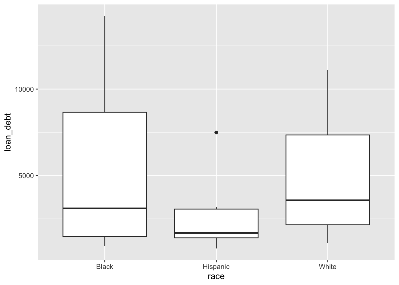
debt |>ggplot() +geom_boxplot(aes(x = race, y = loan_debt))
It’s been 40 years since I saw a box and whisker plot in college… But it’s interesting that Hispanics seem to have lower debt than Blacks and Whites who seem to be about equal.
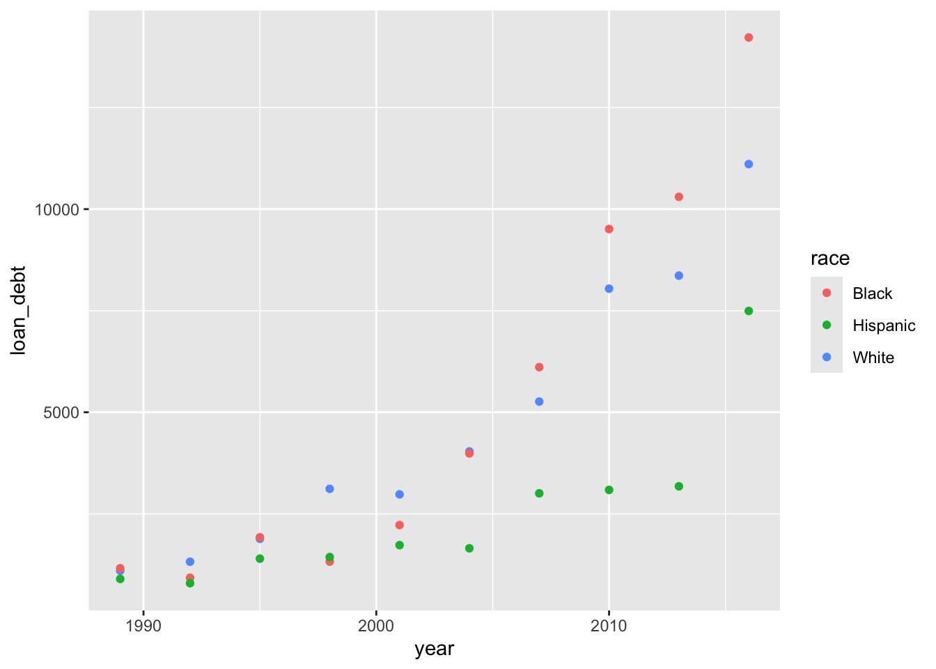
What about debt over time?
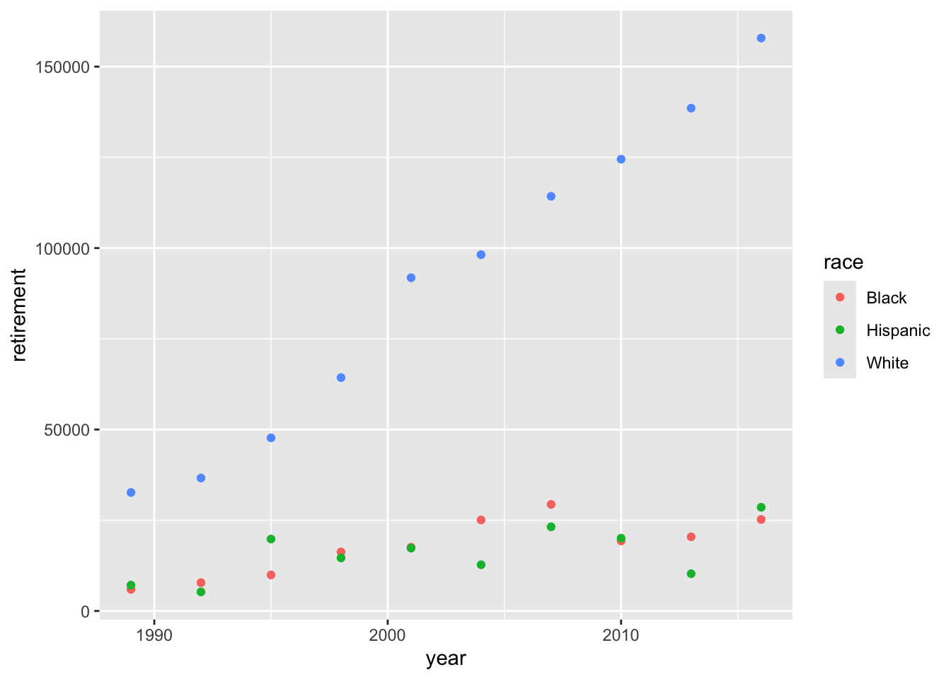
debt |>ggplot() +geom_point(aes(x = year, y = loan_debt, color = race))
The difference in debt between Blacks and Whites increases dramatically over time.
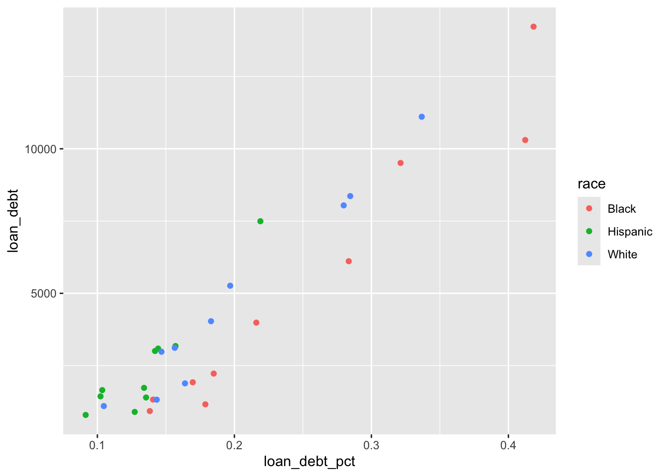
Does the share of families with debt change over time?
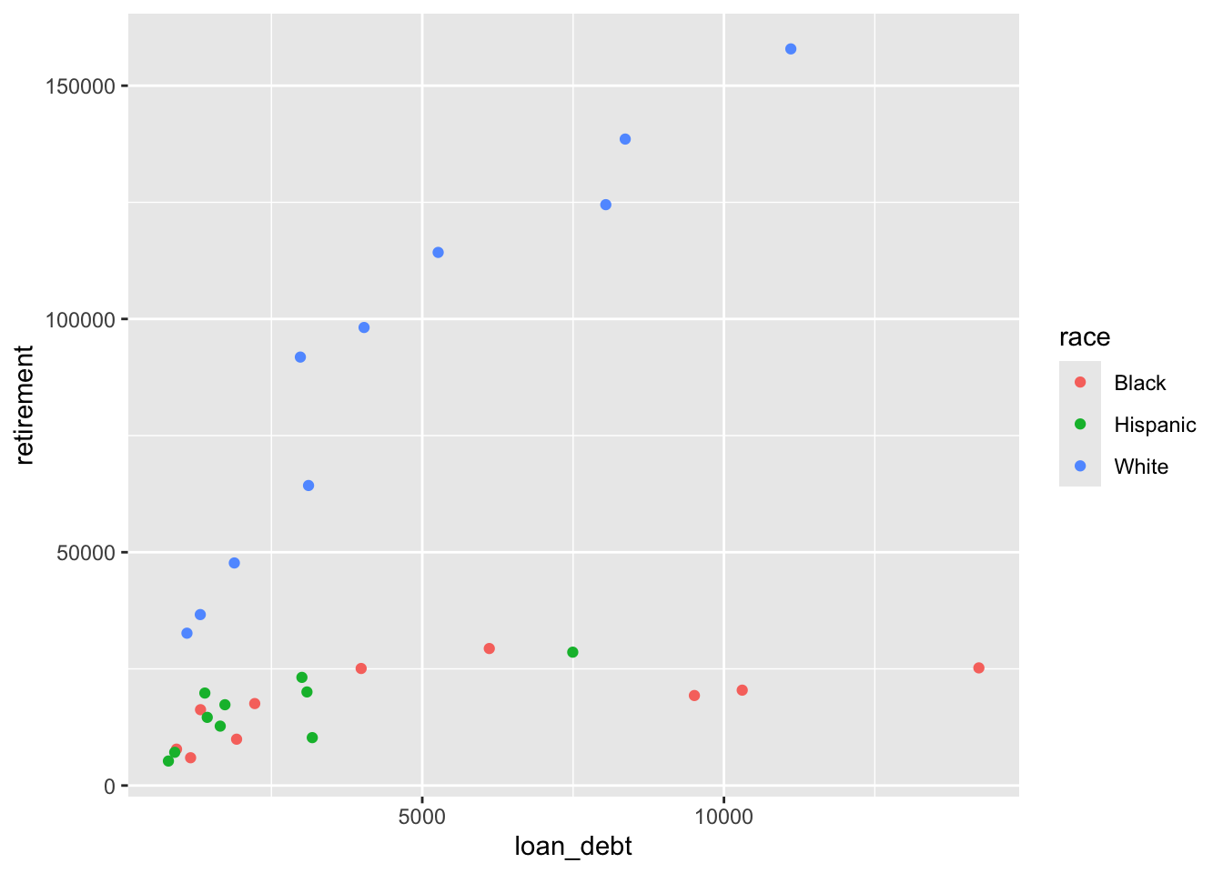
debt |>ggplot() +geom_point(aes(x = loan_debt_pct, y = loan_debt, color = race))
It appears that fewer Hispanics take on student loan debt than Blacks or Whites.
Looking at retirement
Can we copy/paste that code for retirement?
Yes. Yes we can!
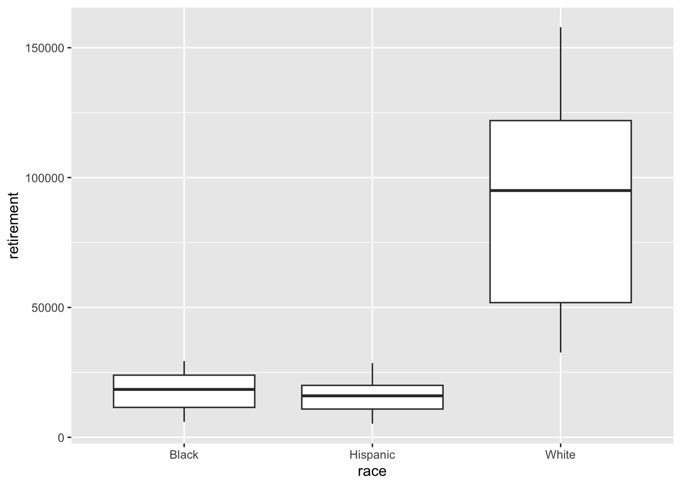
retirement |>ggplot() +geom_boxplot(aes(x = race, y = retirement))
Whites seem to have much more solid retirement savings that Blacks or Hispanics. Even the lowest whisker in the Whites plot seems higher than the highest points in the Black or Hispanics plots.
minMaxRetirement <- retirement |>group_by(race) |>summarise(min =min(retirement), max =max(retirement))minMaxRetirement
# A tibble: 3 × 3
  race        min     max
  <chr>     <dbl>   <dbl>
1 Black     5954.  29365.
2 Hispanic  5249.  28581.
3 White    32649. 157884.
   wealth_type  year      race wealth_family
        <char> <int>    <char>         <num>
1:     Average  1963 Non-White      19503.84
2:     Average  1963     White     140632.66
3:     Average  1963     Black            NA
4:     Average  1963  Hispanic            NA
5:     Average  1983 Non-White      73233.62
6:     Average  1983     White     324057.60
summary(wealth)
 wealth_type             year          race           wealth_family
 Length:96          Min.   :1963   Length:96          Min.   :  2467
 Class :character   1st Qu.:1991   Class :character   1st Qu.: 19559
 Mode  :character   Median :2000   Mode  :character   Median : 97209
                    Mean   :1998                      Mean   :158020
                    3rd Qu.:2008                      3rd Qu.:156895
                    Max.   :2016                      Max.   :919336
                                                      NA's   :24
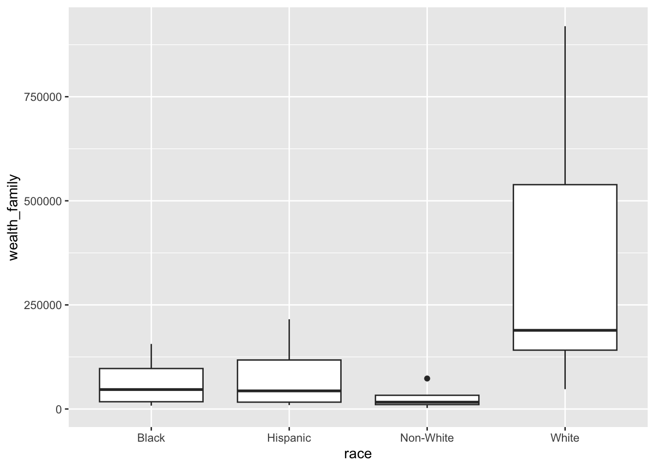
wealth |>ggplot() +geom_boxplot(aes(x = race, y = wealth_family))
Warning: Removed 24 rows containing non-finite outside the scale range
(`stat_boxplot()`).
Oh. That’s interesting. I think family wealth includes all assets and debts, liquid or not. That’s not a great indication of actual wealth.
It looks like there’s some data missing so lets filter for years greater than or equal to 1985 and for the median, rather than average, income.
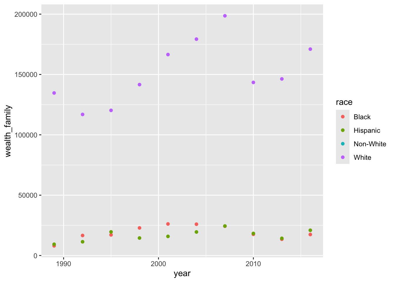
wealth |>filter(year >=1985, wealth_type =="Median") |>ggplot() +geom_point(aes(x = year, y = wealth_family, color = race))
Warning: Removed 10 rows containing missing values or values outside the scale range
(`geom_point()`).
It looks like there isn’t any data for Non-Whites. The median has increased for Whites, but dropped in 2008, while for others it has remained the same over time.
Add wealth into the mix
df <-left_join(debt_retirement, wealth, by =c("race", "year"))head(df)
    year     race loan_debt loan_debt_pct retirement wealth_type wealth_family
   <int>   <char>     <num>         <num>      <num>      <char>         <num>
1:  2016    White 11108.410     0.3367511  157884.20     Average      919336.1
2:  2016    White 11108.410     0.3367511  157884.20      Median      171000.0
3:  2016    Black 14224.770     0.4183588   25211.85     Average      139523.1
4:  2016    Black 14224.770     0.4183588   25211.85      Median       17409.0
5:  2016 Hispanic  7493.999     0.2189689   28581.12     Average      191727.3
6:  2016 Hispanic  7493.999     0.2189689   28581.12      Median       20920.0
It’s kinda confusing with wealth_type, let’s change it a bit
Warning in dewey::regsearch(df, dependent = "retirement", independent =
colnames(df)[c(1:4, : Missing 'interactions' argument. Defaulting to FALSE.
Warning in dewey::regsearch(df, dependent = "retirement", independent =
colnames(df)[c(1:4, : Missing 'multi' argument. Defaulting to FALSE.
[1] "Assembling regresions..."
[1] "Creating 63 formulas. Please be patient, this may take a while."
[1] "Creating regressions..."
[1] "Running 63 regressions. Please be patient, this may take a while."
[1] "Running regressions..."
I would choose retirement ~ + average_wealth + loan_debt + loan_debt_pct + median_wealth because it has the highest \(R^2\) value.
That’s not quite right. retirement ~ + average_wealth + median_wealth is much better because 96% of the model is explained by those two variables so adding loan_debt_pct and loan_debt does not give a lot of benefit.
Warning in dewey::regsearch(df, dependent = "retirement", independent =
colnames(df)[c(1:4, : Missing 'multi' argument. Defaulting to FALSE.
[1] "Gathering variables..."
[1] "WARNING: Using interaction terms without multithreading may take a very long time"
[1] "Assembling regresions..."
[1] "Creating 82159 formulas. Please be patient, this may take a while."
[1] "Creating regressions..."
[1] "Running 14828 regressions. Please be patient, this may take a while."
[1] "Running regressions..."
This is pretty cool. Average wealth by itself is pretty good, but when it interacts with loan_debt_pct, median_wealth, race, and year, it seems to produce a really great model.
Of course, we still want to be careful about overfitting.
Parting Thoughts
Race appears to have a huge impact on everything and increasing educational debt increases retirement, but only for Whites. I’d be curious to see the data behind the loans to learn why increasing educational debt does not always correlate with increased wealth.
Post-Conclusion
It’s Gus again. I had a really fun time with this. I like to think my mom learned a lot and I’m hoping you did too.